
An ink cloud swirling around an obstacle looks like a rendering issue. In reality, the image is the last step of another problem: calculate how a quantity transported moves through a velocity field that must obey physical restrictions. A shader can make the result look liquid; It cannot explain on its own what the algorithm preserves, what it approximates, or why a loss of detail appears.
This paper develops a two-dimensional, incompressible, constant fluid densitymodel, suitable for idealized smoke or ink on a regular grid. Its objective is not to certify a CFD simulator, but to show how a differential equation is converted into operations on arrangements and textures. The approach is supported by Stable Fluids by Jos Stam and GPU development by Mark Harris. The laboratories described arereproducible proposals, not executed results; There are no own FPS, error or performance measurements.
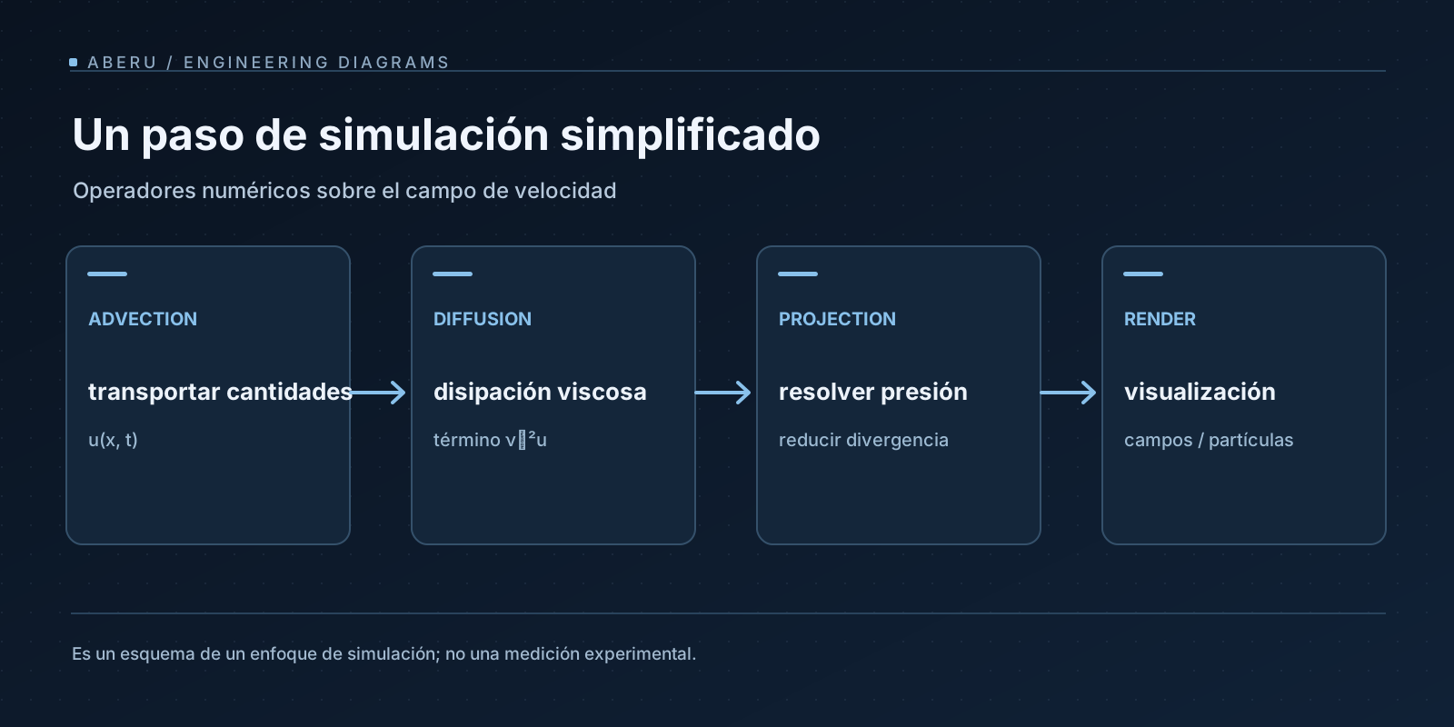
1. What does a cell represent?
In the spatial domain Ω, for each position x = (x, y) and time t, we consider four magnitudes:
| Symbol | Interpretation | Physical unit |
|---|---|---|
| u(x,t) = (u,v) | fluid velocity | m/s |
| p(x,t) | Pressure | Da |
| ρ | Density of fluid, assumed constant | kg/m³ |
| c(x,t) | Ink or smoke concentration; passive tracer | depending on the model |
It is important not to call ρ both the density of the fluid and the color of the ink. In an incomprehensible constant density model, ρ participates in the momentum equation; c is an additional field that the velocity carries. A colored smoke does not mean that we have modeled all the thermodynamics of a gas.
On a uniform grid we store discrete values u[i,j], v[i,j], p[i,j] and c[i,j]. The horizontal step is Δx, the vertical step is Δy, and each update advances Δt. If velocity lives in cell centers, particular difficulties appear in deriving fields; A step grid (MAC) places velocity components on faces and pressure on centers to better couple divergence and gradient. The choice is not just a detail of memory: it determines the formulas that preserve discrete identities.
2. The equations and their meaning
For velocity u, constant density, kinematic viscosity ν and external acceleration f, the incompressible Navier–Stokes equation is written:
∂u/∂t + (u · ∇)u = −(1/ρ)∇p + ν∇²u + f
∇ · u = 0
Each operator imposes a different responsibility:
- Temporal derivative: how the velocity changes at a fixed position.
- Advection
(u · ∇)u: how the flow itself carries its velocity. ∇ppressure gradient: pressure difference that accelerates the fluid.- Laplacian
∇²u: velocity diffusion due to viscosity. ∇ · udivergence: local net flow. For incompressibility it must be zero.
In two dimensions ∇ · u = ∂u/∂x + ∂v/∂y. For a scalar q, ∇q = (∂q/∂x, ∂q/∂y) and ∇²q = ∂²q/∂x² + ∂²q/∂y². The material derivative D/Dt = ∂/∂t + u · ∇ brings together temporal change and transportation.
The tracer equation, without sources or molecular diffusion, is different:
∂c/∂t + u · ∇c = 0
If a diffusivity κ and a source s are modeled, it becomes ∂c/∂t + u · ∇c = κ∇²c + s. Not pressure is another color that is advecua: it works as a multiplier that imposes the null divergence constraint.
3. From derivatives to finite differences
A derivative is a limit; a GPU needs samples. On a centered grid, far from boundaries, the central derivative and the 2D Laplacian can be approximated like this:
∂q/∂x  ≈ (q[i+1,j] − q[i−1,j]) / (2Δx)
∂q/∂y  ≈ (q[i,j+1] − q[i,j−1]) / (2Δy)

∇²q ≈ (q[i+1,j] − 2q[i,j] + q[i−1,j]) / Δx²
     + (q[i,j+1] − 2q[i,j] + q[i,j−1]) / Δy²
They are approximations of order two in space for sufficiently smooth fields, not promises of global precision of the solver: advection, iterative resolution, edges and temporal discretization provide other errors. If Δx ≠ Δy, using a single Δx² divisor in both directions is a bug, not an innocent simplification.
To update the equations, operator splitting is applied: solve advection, forces, diffusion and pressure separately, and combine the result of each substep. There is no single universal order. In Stam’s classical formulation, velocity is diffused, then advected and projected; some implementations reorder substeps or project more than once. Each variant modifies the separation error and must be documented as such.
4. Advection: asking where the fluid came from
The semi-Lagrangian method does not actively push each particle to a future cell. For each target sample x, back in the speeds field and refer to the previous state:
x_back ≈ x − Δt · u_old(x)
q_new(x) = interpolate(q_old, x_back)
This is a first order approximation for the trajectory. Position integration can be improved—for example, with a midpoint—without automatically converting the entire scheme to a second-order one: spatial interpolation also matters. In a 2D texture, bilinear interpolation combines the four neighboring texels. Samples outside the domain must be explicitly defined: clamp, reflection, periodic boundary or obstacle treatment.
The advantage is practical: classical semi-Lagrangian advection with stable interpolation avoids the strict advective CFL restriction of many explicit schemes. The cost appears elsewhere: it loses sharpness and does not exactly preserve the tracer integral. By repeatedly interpolating, a spot can blur even though the continuous equation does not include diffusion. ∑c can vary even when the speed is approximately solenoidal; correcting divergence does not by itself repair this non-conservative transport.
Therefore, “stable for large steps” does not mean “physically correct for any Δt”. Excessive stepping can erase structures, traverse obstacles if features are not treated correctly, or introduce large trajectory errors.
5. Diffusion: a hidden linear equation
To represent viscosity in isolation we solve for ∂u/∂t = ν∇²u. An implicit temporal discretization gives:
(I − νΔt L) u_new = u_old
Here L is the discrete Laplacian operator. On a uniform grid with Δx = Δy = h, defining a = νΔt/h², an interior Jacobi iteration results:
u_new[i,j] = (u_old[i,j] + a · (u_iter[i+1,j] + u_iter[i−1,j]
                    + u_iter[i,j+1] + u_iter[i,j−1])) / (1 + 4a)
The formula of each component is evaluated on an iteration buffer, always reading from the previous iteration; Gauss–Seidel on CPU can update in another order. A fixed number of iterations is a cost policy, not a convergence test. The residual of the linear system must be measured if we need numerical guarantees.
An explicit approximation also exists, but imposes stability restrictions related to νΔt/h². The implicit approach is especially useful when it is important to tolerate larger steps without explosions caused by diffusion.
6. Projection: resolve pressure to correct divergence
After forces, diffusion and advection we have an intermediate velocity u* that generally does not exactly satisfy ∇ · u* = 0. We are looking for a p pressure to build:
u_next = u* − (Δt/ρ)∇p
Applying divergence and imposing ∇ · u_next = 0, we obtain the Poisson problem:
∇²p = (ρ/Δt) · (∇ · u*)
On a square grid of spacing h, the inner Jacobi update has the form:
p_new[i,j] = (p_old[i+1,j] + p_old[i−1,j]
            + p_old[i,j+1] + p_old[i,j−1] − h² · rhs[i,j]) / 4
rhs is (ρ/Δt) div(u*). We then subtract the discrete pressure gradient from u*. A crucial property for the implementation is to use compatible divergence, gradient and Laplacian operators. If the Laplacian of the solver does not correspond to the discrete composition of gradient and divergence applied in the correction, the Poisson residual alone does not predict the final divergence.
Furthermore, Jacobi solved with finite iterations only approximates the solution. With Neumann boundaries, the pressure is determined up to a constant: fixing a pressure reference or eliminating the mean helps deal with the null space. Solvability conditions and imposed normal flow also matter. A discrete projection reduces, but does not guarantee to literally bring all divergences to zero with arbitrary tolerance.
What to really measure
It is not enough to count iterations. In the laboratory I would record two different observables:
residuo_Poisson = ||L p − rhs||₂
error_div       = ||D(u_next)||₂
D is the discrete divergence used by the solver. It is also advisable to report the absolute maximum and relative norm, specify how the solid cells are treated, and record the cost of the projection step. Arbitrary values like 1e-5 lack universal meaning without scaling, resolution, precision, and normalization.
7. Borders: there you can see the difference between demo and solver
An impermeable wall imposes zero normal velocity, u · n = 0. The no slip condition adds that the tangential velocity is zero; free slip allows tangential movement with the right condition. Periodic boundaries require neighbors on opposite sides to share the correct topology and operators. Poisson usually uses conditions derived from the normal velocity condition, not an indiscriminate p=0 on each wall.
An obstacle mask changes the local stencil: solid cells should not be treated simply as liquid with zero visual density. If an obstacle cuts an edge, pressure, hindcast advection, and divergence calculation must agree on where the fluid domain begins.
To debug, I would start with an empty case with zero velocity, a periodic uniform field, a localized impulse, and a tracer displaced in a uniform field. Only later would I add walls and fountains. The goal is to isolate errors before a nice cloud hides them.
8. CPU, WebGL2 and WebGPU: three execution models
The algorithm operates on fields; It doesn’t prescribe your hardware. In CPU we can keep flat arrays or a MAC grid and use clear loops, useful as a correction reference. On GPU, one advection pass becomes the texture sampling per output texel; Jacobi is equivalent to many passes of the same kernel with alternating inputs and outputs.
In WebGL2those kernels are typically implemented as fragment shaders that render textures in framebuffers. WebGL2 does not incorporate general compute shaders. The ability to render in floating point textures and filter those formats depends on device capabilities and extensions; must be verified in runtime. Compute passes with buffers or storage textures can be used onWebGPU, but availability and effective limits also depend on the browser, adapter, and device.
The ping-pong pattern maintains two physical resources: read A, write B, swap them, repeat. Avoid relying on incompatible simultaneous reads and writes to the same resource. Each stage has a dispatch/pass cost and memory traffic. A pressure solver with k iterations and N cells requires, conceptually, O(kN) arithmetic work and memory access; The actual time depends on bandwidth, overhead, cache and synchronization.
Choosing GPU because “a field is parallel” is not enough. A small grid, frequent CPU↔GPU transfers, limited resolution, or many barriers can make the CPU solution more desirable. For comparison, I would measure advection, diffusion, pressure, transfer and render time separately, with warm-up and repeated measurements. No numerical results are provided here.
9. A documentable simulation cycle
A possible didactic pipeline is the following; The order should remain fixed between experiments:
estado anterior: velocidad u, trazador c
  1) incorporar fuerzas externas en u
  2) difundir u implícitamente (si ν > 0)
  3) advectar u usando el campo elegido
  4) calcular D(u*) y resolver Lp = (ρ/Δt)D(u*)
  5) corregir u* con el gradiente de p
  6) advectar c con la velocidad proyectada
  7) aplicar fuentes/sumideros explícitos de c (si existen)
  8) visualizar c; inspeccionar residual y divergencia
The sequence is an editorial scheme. It does not by itself contain the details to run a solver: it is missing stencils, barriers, precision, parameters, corner treatment and edge contracts. It is also possible to project before other stages, implement a higher order method or use staggered grids. These decisions must be documented to compare two implementations without attributing changes caused by several to one factor.
10. Validation protocol without invented benchmarks
I would design a test array with grid size N ∈ {64, 128, 256}, small/medium/large Δt defined in consistent units, and different Poisson iterations; all tests would keep initial conditions and boundary rules the same. The metrics would be divergence error, Poisson residual, total tracer variation, c center of mass position, discrete kinetic energy, cost per substep, and memory.
**Case A — rest:**zero speed and absence of forces; The state should remain idle up to numerical tolerance.**Case B — periodic uniform advection:**transport a smooth distribution and compare its displacement with the analytical translation; here amplitude losses appear due to interpolation.**Case C — synthetic non-solenoidal field:**measure divergence decrease when projecting.**Case D — resolution:**repeat with decreasing h maintaining physical magnitudes and compare error, not just images.Case E — barriers: verify that there is no normal speed to the wall outside the tolerance.
It is not appropriate to assume that ∑c is exactly constant because it is incompressible nor that doubling the iterations guarantees a proportional gain. In particular, any claim of “60 FPS” or CPU/GPU improvement requires hardware, resolution, texture format, browser version, warm-up criteria, and an actual test log. The dossier proposes these measurements; has not executed them.
11. What changes when pursuing visual detail
Vorticity confinement adds a force calculated from local rotation to return structure to eddies attenuated by discretization. It may improve appearance, but introduces energy that does not necessarily come from the original physical model. Increasing resolution, using higher order interpolation or applying antidiffusion corrections also changes stability and cost. A more dramatic image is not automatically a more accurate simulation.
The central distinction is this: the continuous equation expresses conservation and dynamics; the discrete method expresses an approximation; The render expresses a visual interpretation of the field. Designing a real-time solver is about making trade-offs explicit and measuring the properties that really matter for your goal.
Readings and primary sources
- Jos Stam — Stable Fluids (SIGGRAPH, 1999), publicaciones del autor. Foundation of the semi-Lagrangian advection approach and operator separation.
- Jos Stam — Real-Time Fluid Dynamics for Games (GDC, 2003). Pedagogical presentation of the scheme and its implementation.
- Mark J. Harris — Fast Fluid Dynamics Simulation on the GPU, GPU Gems, capítulo 38. Discretization, boundaries and GPU steps.
- MDN — WebGL2RenderingContext. WebGL 2 context capabilities.
- MDN — WebGPU API. Availability, compute model and platform restrictions.
Predicted visual extensions: Navier–Stokes term decomposition, semi-Lagrangian trajectory, and before/after divergence comparison. The cover page and the conceptual diagram of the solver are already incorporated; no interactive simulation or measured results are presented. Targets for additional figures follow at docs/BLOCK-08-FIGMA-SHOTLIST.md.
Additional animation: simulación 2D de la estela de vórtices de Kármán (Tensorion, CC BY 4.0). The original external file is larger than 20 MB; links instead of preloading it as a cover.

