
When a route appears on a map it seems that the algorithm has “seen” corridors, walls and destinations. It’s not like that. The algorithm sees a graph: vertices, edges, costs and, sometimes, an estimate of how far to go. The visual representation is a projection of those decisions. A flashy search animation does not prove that the result is optimal; A correct data structure does allow you to reason why it should be.
This article compares BFS, Dijkstra and A* using the same grid search problem, but preserving the mathematical conditions that make their guarantees valid. The laboratory is a test specification; comparisons of time, memory and number of expansions have not been measured. The central pedagogical reference is Introduction to the A Algorithm*, de Amit Patel, complemented by graph theory and path-finding algorithms.
1. The map is not the graph
A graph G = (V, E) contains a set of vertices V and edges E. In a grid, we can represent each traversable cell (x, y) as a vertex; edges connect cells between which movement is allowed. Drawing the cells does not define the edges. Two visually identical maps can induce different graphs if one allows diagonals, another prohibits crossing corners, or assigns different costs to terrain and movements.
Let’s consider a square board. With four-neighbor connectivity, from (x,y) we can move to (x±1,y) or (x,y±1), as long as the destination is valid. If we add diagonals, there are now four more edges per cell. The usual cost of an orthogonal step may be 1 and the diagonal √2, but they are modeling choices. If both addresses cost 1, the optimal problem changes and the admissible heuristic changes.
A wall can block vertices, edges, or both. In particular, moving diagonally between two locked orthogonal cells constitutes corner cutting; Allowing or preventing it should be an explicit policy, not an accidental effect of the neighbor loop. To compare algorithms, the graph and the movement rules have to be identical.
Edge weight and node cost
Dijkstra and A* minimize the sum of edge weights in a path. A cost associated with terrain can be converted into a cell entry cost or an average of the costs of both cells, but each transformation changes the interpretation. If dangerous terrain costs 5 and normal terrain costs 1, the route with fewer steps may be more expensive than a longer loop.
Let’s not confuse the geometric length (meters), number of steps and added cost (time, energy, risk). If the UI presents “shortest path” you must clarify in which metric.
2. BFS: the distance by number of edges
Breadth-First Search explores by layers of depth. It starts with the source in a FIFO queue and records when it first discovers a neighbor. All vertex distance d edges are discovered before any vertex distance greater. This property is proven by induction on the queue extractions.
cola ← [inicio]
visitados ← {inicio}
padre[inicio] ← ninguno

mientras cola no esté vacía:
    actual ← quitar_primero(cola)
    si actual = meta: terminar con éxito
    para vecino de actual, en orden estable:
        si vecino no está bloqueado y vecino no fue visitado:
            visitados.agregar(vecino)
            padre[vecino] ← actual
            agregar_al_final(cola, vecino)
BFS is complete on a finite graph and obtains a path with the minimum number of edges; only minimizes total cost if all relevant edges have the same positive cost. If costs vary, the closest layer is not the cheapest. Its time cost is O(V + E) with adjacency lists and FIFO structure; O(V) requires space for visited, predecessors and queue in the worst case.
The typical display is a nearly concentric wave: coloring a vertex as “uncovered” when it enters the queue and as “expanded” when it exits. These two states are not equivalent. The boundary does not represent already closed nodes; This is what remains to be expanded.
3. Dijkstra: choose the smallest confirmed cost
If the edges have non-negativeweights, BFS no longer has the correct layers property. Dijkstra replaces the FIFO with a minimum priority queue and maintains a tentative distance g(v) for each vertex. Initialize g(inicio) = 0 and the rest to infinity. Every time it finds a cheaper path to v, it performs therelaxation operation:
si g(u) + peso(u, v) < g(v):
    g(v) ← g(u) + peso(u, v)
    padre[v] ← u
    insertar_o_actualizar(v, prioridad = g(v))
When we extract a node with the smallest valid tentative distance and its edges are non-negative, that distance can be considered final. The justification is simple: any alternative route that still passes through a pending vertex cannot accumulate less cost if all its future increments are non-negative.
In a practical implementation with heapq or priority_queue, a new entry is usually inserted instead of decrementing an existing key. Therefore, there may be obsolete duplicates in the heap. We must discard entries whose cost no longer matches the best known or nodes that have been definitively expanded. Pseudocode without this check hides a real implementation problem.
With binary heap, the typical complexity is expressed O((V + E) log V) for a priority update implementation; The precise dimensions change when there are duplicate insertions (log E) and depending on how vertices are represented and operations are counted. In sparse E = O(V) grids, both notations simplify to order O(V log V).
Counterexample to BFS: from S there is a direct edge to G of cost 10, and another to A of cost 1, followed by A → G of cost 1. BFS chooses the path of an edge; Dijkstra finds the cost 2. It’s not a BFS bug: it was applied to a different target than the one it resolves.
Dijkstra is not appropriate for negative edges in its usual formulation. If the network contains negative costs, you must first review what the metric means and whether a negative cost cycle exists; In general cases, other algorithms are needed, such as Bellman–Ford. Don’t try to “fix” it by turning off distance validations.
4. A*: use information without sacrificing correctness
A* adds an estimate of the cost from each node to the goal, called h(n). Sort the border by:
f(n) = g(n) + h(n)

g(n) = coste mínimo encontrado desde el origen hasta n
h(n) = estimación del coste restante de n a la meta
If h(n) = 0 for all nodes, A* behaves like Dijkstra with possible tie-breaking differences. With a useful estimate, first look for promising states without ignoring what it already took to get there.
The important word is allowable: for each node, h(n) must not overestimate the minimum remaining actual cost h*(n). Thus, h(n) ≤ h*(n). A heuristic is consistent if h(u) ≤ w(u,v) + h(v) for each edge u → v, and h(meta)=0. Consistency implies admissibility in standard cases and allows g values of closed nodes to be treated as final.
With an admissible but inconsistent heuristic, A* with graph search can still be optimal if it reopens nodes when it discovers better paths and properly handles termination. The statement “it is enough that h is admissible” is incomplete when the implementation prohibits reopening states. For the example in this article we will use consistent heuristics and non-negative costs.
What heuristics correspond to each grid
Let dx = |x_meta − x| and dy = |y_meta − y|, with cell length 1 and cost per unit distance of at least 1:
| Allowed movement | Cost | Usual heuristic |
|---|---|---|
| Only four directions | Each step 1 | Manhattan: dx + dy |
| Eight directions | Diagonal also 1 | Chebyshev: max(dx,dy) |
| Eight directions | Straight 1, diagonal √2 | Octile: dx + dy + (√2 − 2) min(dx,dy) |
| Free geometric distance | Cost at least Euclidean distance | Euclidean: sqrt(dx² + dy²) |
Each formula assumes the indicated rules and weights. With weighted terrain whose minimum cost per unit distance is c_min > 0, a geometric heuristic can be multiplied by c_min to preserve a lower bound. With zero costs, multiplying by a zero minimum gives a trivial but safe heuristic. Do not simply use Manhattan on a grid of eight neighbors: When the diagonal costs 1 or √2, Manhattan may overestimate the available route.
A heuristic multiplied by w > 1 is known in variants as Weighted A*; It can reduce explorations in certain scenarios in exchange for abandoning the strict optimality guarantee, except for additional guarantees of the specific variant. That variant should not be mixed with an admissible A* in an unlabeled benchmark.
5. A reference kernel in Python
The following snippet implements priority-guided search over a finite explicit graph, with non-negative weights, discarded stale entries, and implicit reopening when g improves. With heuristic = 0 it acts as Dijkstra; with a suitable allowable heuristic is used as A*. Does not generate views; returns path, cost and number of expansions for instrumentation. In a general graph with inconsistent heuristics, the implementation termination conditions must also be examined.
import heapq
import itertools
import math


def shortest_path(graph, start, goal, heuristic=lambda node: 0.0):
    best = {start: 0.0}
    parent = {start: None}
    counter = itertools.count()
    queue = [(heuristic(start), next(counter), 0.0, start)]
    expanded = 0

    while queue:
        _priority, _seq, cost, node = heapq.heappop(queue)
        if cost != best.get(node, math.inf):  # entrada obsoleta
            continue
        expanded += 1
        if node == goal:
            path = [node]
            while parent[node] is not None:
                node = parent[node]
                path.append(node)
            return list(reversed(path)), cost, expanded

        for neighbor, weight in graph.get(node, ()):
            if not math.isfinite(weight) or weight < 0:
                raise ValueError("Se requieren pesos finitos no negativos")
            candidate = cost + weight
            if candidate < best.get(neighbor, math.inf):
                best[neighbor] = candidate
                parent[neighbor] = node
                priority = candidate + heuristic(neighbor)
                heapq.heappush(
                    queue, (priority, next(counter), candidate, neighbor)
                )
    return None, math.inf, expanded
Tiebreaking using counter avoids relying on nodes being comparable. Using exact equality to detect a stale entry is appropriate here because the same candidate value calculated when inserting it is stored; it is not a general test of numerical equality between two independent calculations. Furthermore, the algorithm does not replace graph validations, termination policies under inconsistent heuristics, or a unit optimality test. Your example contract is: finite graph, non-negative weights, consistent heuristic and heuristic(meta)=0.
In an implementation with additional capabilities one event can be saved per transition: discover, decrease, expand, goal. These traces allow the border images to be reproduced without mixing animation time with search time.
6. The path is a tree of predecessors, not a list that appears alone
Both BFS, Dijkstra and A* can reconstruct the result by storing parent[v] when they discover or improve a route. From the goal, the parents are traversed to the origin and the sequence is reversed. If source and goal are the same node, the response contains only that node with zero cost. If the target is inaccessible, the algorithm explicitly returns “no route”; not an empty path that the UI can interpret as success.
A graph can have several optimal paths. The neighbor order, insertion order, and tiebreaking rule can change which one is returned, even if the cost is identical. In an animation, two executions with different paths do not mean that one is incorrect. For visual reproducibility, set order of neighbors and tiebreakers.
7. What “faster” means in a visualization
There are at least four different measurements:
- Expanded nodes: how many states validly left the border and were processed.
- Maximum boundary: Maximum size of the logical queue or physical heap, including whether stale entries are counted.
- Search Time: No cell painting, animation, or browser event latency.
- Path cost: exact sum of the edge weights of the reconstructed route.
A* does not always expand fewer nodes than Dijkstra in any graph or implementation; heuristics, tiebreakers, obstacles and costs influence. A poorly scaled heuristic can give an incorrect result if admissibility is lost. We also cannot compare times from an animation with one artificial visual step per node.
Asymptotic complexity is not a prediction of seconds. BFS has the limit O(V+E) and is appropriate when costs are uniform. Dijkstra uses a heap for cost order. A* uses the same machinery with an estimate and its memory usage can still be large; A perfect heuristic does not make neighbor generation or the boundary cost trivial in all problems.
8. Design a comparable laboratory
I would propose a set of boards with seed and fixed obstacles, sizes from 50×50 to 500×500, three movement rules and two cost distributions. Each run would record board hash, source/goal, algorithm version, tiebreaker policy, heap type, hardware, warm-up, and repetitions. The following scenarios separate different questions:
| Scenery | Valid comparison | Expected invariant |
|---|---|---|
Grid of four neighbors and cost 1 | BFS / Dijkstra / A* Manhattan | Same optimal cost, not necessarily same path |
| Land with positive variable costs | Dijkstra / A* with admissible heuristics | Same optimal cost |
Eight neighbors, diagonal √2 | Dijkstra / A* octile | No heuristic overestimation |
h = 0 | Dijkstra / A* | Equal cost and equivalent exploration except tiebreakers |
| Inaccessible goal | All three, under valid rules | “No route” result |
| Origin = goal | The three | 0 cost, one node |
It is crucial to compare cost and not just route length. In a weighted map, an optimal route can visit more nodes than an expensive route. For visual evaluation, we would retain three layers: obstacle/walkability; discovered/border/expanded; and final route. The UI should distinguish real calculation time and artificial animation time, and allow pausing without altering the order of the algorithm.
An additional property test would generate small random graphs with non-negative weights. Dijkstra would be the oracle to verify the cost produced by A* with consistent heuristics; in graphs with unit weights BFS would serve as another oracle. This detects errors that a single maze demo would never reveal.
9. Where does this model end?
Grids are convenient for teaching, but a real world can be represented with navigation meshes, hierarchical regions, road graphs, costs that change over time, and bodies with different sizes or radii of gyration. A* on the graph we give you does not automatically resolve continuous collisions or cooperative movements. A character can follow a topologically valid path and physically collide if its dimensions are not modeled.
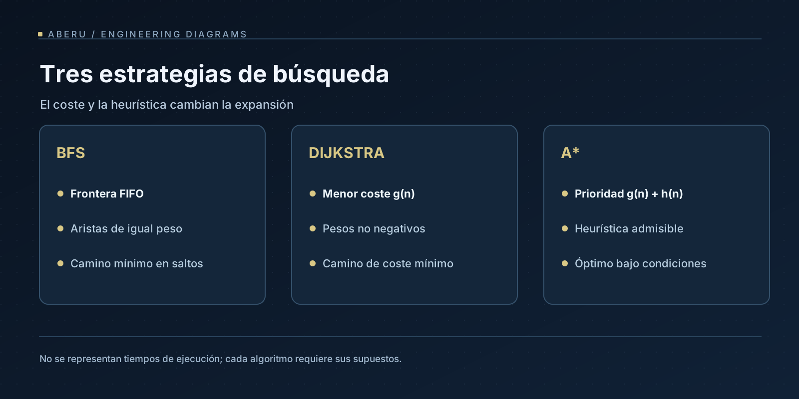
All three algorithms answer precise questions. BFSminimizes edges with uniform costs;Dijkstraminimizes non-negative weights without needing a meta heuristic;A*combines observed cost with a lower bound for heading to the goal. Visualizing them helps to understand your search, as long asthe visualization respects the graph and the invariants.
Readings and sources
- Amit Patel — Introduction to the A Algorithm*. Graph model, boundaries, reconstruction and interactive comparison.
- Amit Patel — Implementation of A. Data structures and implementation decisions.
- Amit Patel — Heuristics. Manhattan distances, octile and guarantees.
- MIT OpenCourseWare — Introduction to Algorithms. Formal basis for search, graphs and priorities.
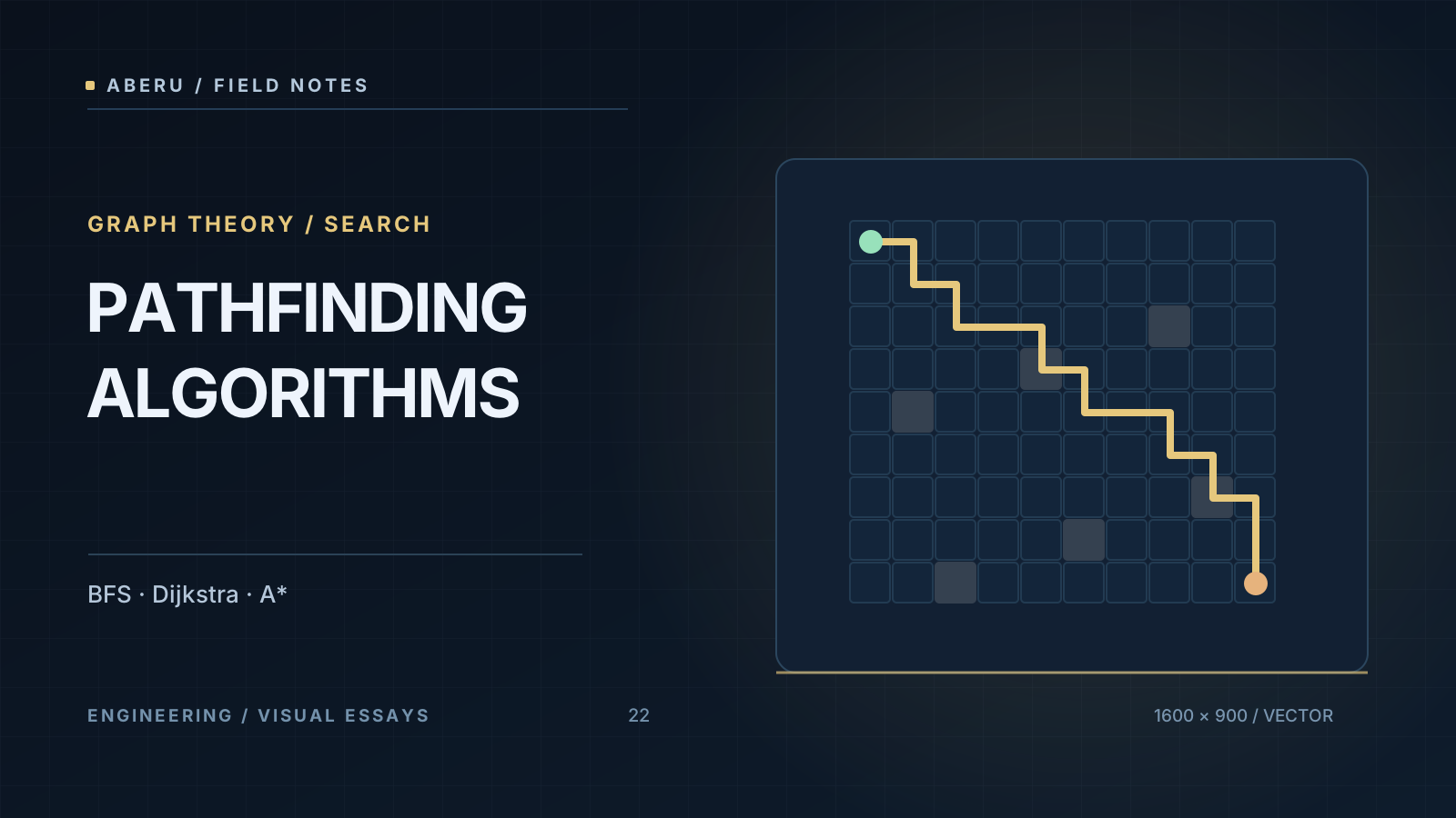
Future visual expansions: Animated comparisons of borders, g/h/f nodes, path reconstruction and diagonal cases. The cover and comparison diagram are now available; An interactive viewer has not yet been developed.
